Question
Answer
The regression equation Y=a+bXY = a + bX is calculated as follows:
b = 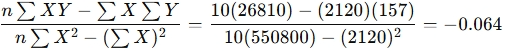
a = 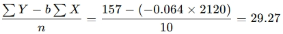
Thus, the regression equation is:
Y = 29.27 − 0.064X
(i) When X=280X the number of errors is:
Y = 29.27 − 0.064 (280) = 11.35
Therefore, a student studying for 280 minutes would make approximately 11 errors.
(ii) The expected change in the number of errors for a 1-minute change in study time is given by the regression coefficient b=−0.064b
Thus, a 1-minute change in study time is expected to result in a 0.064 fewer errors.
(iii) The formula for the Pearson Product Moment Correlation Coefficient rr is:
r = 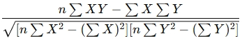
Substituting the given values:
r = 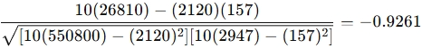
Thus, the Pearson Product Moment Correlation Coefficient is -0.9261.
(iv) The coefficient of determination is calculated as:
![]()
The coefficient of determination is 85.77%, which means 85.77% of the variation in the number of errors made can be explained by the study time.