
Question
Answer
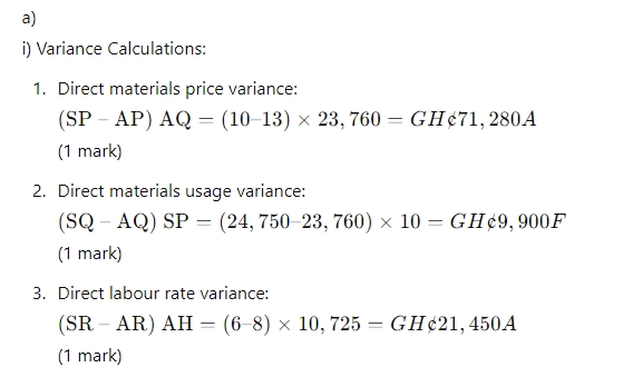
- Possible reason for the material price variance: Increase in raw material prices due to inflation or shortage of materials. (1 mark)
- Possible reason for the labour rate variance: Increase in wage rates due to higher demand for skilled labour or overtime payments. (1 mark)
b) i) Total cost model using high-low method:
| Period | V | TC (GH¢) |
|---|---|---|
| 2 | 515 | 90,275 |
| 1 | 420 | 82,200 |
Change in TC = 90,275 – 82,200 = 8,075 Change in V = 515 – 420 = 95 Variable cost per valuation = 8,075 / 95 = 85
Fixed cost = TC – (VC × V) Using Period 2: Fixed cost = 90,275 – (85 × 515) = 46,000
Total cost model: TC = 46,000 + 85V (4 marks)
ii) Usefulness of the high-low method:
- Simple and Easy: The high-low method is straightforward and easy to apply for estimating fixed and variable costs.
- Limited Data Requirement: Requires only two data points, making it useful when limited data is available.
- Quick Estimates: Provides quick estimates of cost behavior which can be useful for preliminary analysis.
- Potential Issues: However, it ignores data between the high and low points, potentially leading to inaccuracies if those points are not representative of normal operations. Historical data used may not reflect current conditions. (4 marks)
c) Models used to estimate seasonal variations:
- Additive Model:
- Assumes that seasonal variations above and below the trend line in each cycle add up to zero.
- Steps:
- Calculate the difference between the moving average value and the actual historical figure for each time period.
- Group these seasonal variations into different seasons (e.g., days of the week, months, or quarters).
- Calculate the average of these seasonal variations for each season.
- If the total seasonal variations for the cycle do not add up to zero, spread the difference evenly across each season.
- The adjusted figure is the seasonal variation. (3.5 marks)
- Proportional (Multiplicative) Model:
- Expresses the actual value in each season as a proportion of the trend line value.
- Steps:
- Calculate seasonal variations for each time period by dividing the actual data by the corresponding moving average or trend line value.
- Sum of the proportions for each time period must add up to 1 (or the sum of proportions for quarterly data must sum to 4).
- If the sum does not match, spread the difference evenly over each quarter to adjust the proportions. (3.5 marks)